
공부중
Noise Analysis in Operational Amplifier Circuits (4) Noise Characteristics 본문
Noise Analysis in Operational Amplifier Circuits (4) Noise Characteristics
복습 2026. 6. 7. 18:19
Noise Characteristics
노이즈 특성
Since noise sources have amplitudes that vary randomly with time, they can only be specified by a probability density function. Thermal noise and shot noise have Gaussian probability density functions. The other forms of noise noted do not. If \sigma is the standard deviation of the Gaussian distribution, then the instantaneous value lies between the average value of the signal and \pm\sigma 68% of the time.
노이즈원은 시간에 따라 무작위로 변하는 진폭을 가지기 때문에, 오직 확률 밀도 함수(probability density function)로만 규정할 수 있습니다. 열 잡음과 산탄 노이즈는 가우시안(정규) 확률 밀도 함수를 가집니다. 앞서 언급한 다른 형태의 노이즈들은 그렇지 않습니다. 가우시안 분포의 표준편차가 \sigma(시그마)라면, 순간값은 68%의 확률로 신호의 평균값과 \pm\sigma 사이에 위치합니다.
By definition, \sigma^2 (variance) is the average mean-square variation about the average value. This means that in noise signals having Gaussian distributions of amplitude, the average mean-square variation about the average value, i^2 or e^2, is the variance \sigma^2, and the rms value is the standard deviation \sigma.
정의에 따르면, 분산(\sigma^2)은 평균값 주변의 평균 제곱 변동(mean-square variation)입니다. 즉, 진폭이 가우시안 분포를 따르는 노이즈 신호에서 평균값 주변의 평균 제곱 변동인 i^2 또는 e^2은 분산 \sigma^2과 같고, 실효값(rms value)은 표준편차 \sigma와 같습니다.
Theoretically the noise amplitude can have values approaching infinity. However, the probability falls off rapidly as amplitude increases. An effective limit is \pm3\sigma, since the noise amplitude is within these limits 99.7% of the time. Figure 1 shows graphically how the probability of the amplitude relates to the rms value.
이론적으로 노이즈 진폭은 무한대에 가까운 값을 가질 수 있습니다. 그러나 진폭이 증가함에 따라 확률은 급격히 떨어집니다. 노이즈 진폭이 99.7%의 확률로 이 한계 내에 존재하므로, 실질적인 한계는 \pm3\sigma입니다. 그림 1은 진폭의 확률이 rms(실효)값과 어떻게 연관되는지를 시각적으로 보여줍니다.
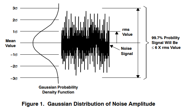
99.7% Probability Signal Will Be \le 6 \times rms Value
99.7%의 확률로 신호가 \le 6 \times rms 값 내에 존재함
Figure 1. Gaussian Distribution of Noise Amplitude
그림 1. 노이즈 진폭의 가우시안 분포
Since the rms value of a noise source is equal to \sigma, to assure that a signal is within peak-to-peak limits 99.7% of the time, multiply the rms value by 6 (+3\sigma − (−3\sigma)): Erms \times 6 = Epp. For more or less assurance, use values between 4 (95.4%) and 6.8 (99.94%).
노이즈원의 rms 값은 \sigma와 같으므로, 신호가 99.7%의 확률로 최대-최대(peak-to-peak) 한계 내에 있도록 보장하려면 rms 값에 6을 곱해야 합니다 (+3\sigma − (−3\sigma)): Erms \times 6 = Epp. 더 높거나 낮은 신뢰 수준을 원한다면 4 (95.4%)에서 6.8 (99.94%) 사이의 값을 사용할 수 있습니다.
Adding Noise Sources
노이즈원 합산하기
With multiple noise sources in a circuit, the signals must be combined properly to obtain the overall noise signal.
회로 내에 여러 노이즈원이 존재하는 경우, 전체 노이즈 신호를 구하기 위해 각 신호들을 올바르게 결합해야 합니다.
Consider the example of two resistors, R1 and R2, connected in series. Each resistor has a noise generator associated with it as shown in Figure 2 where e_1^2 = 4kTR1df and e_2^2 = 4kTR2df.
직렬로 연결된 두 저항 R1과 R2의 예시를 살펴보겠습니다. 각 저항에는 그림 2에 나타난 것과 같이 e_1^2 = 4kTR1df 및 e_2^2 = 4kTR2df인 노이즈 발생기가 결합되어 있습니다.

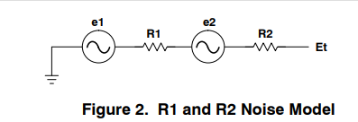
To calculate the average mean square voltage, E_t^2, across the two resistors, let E_t(t) = e_1(t) + e_2(t) be the instantaneous values. Then
E_t(t)^2 = (e_1(t) + e_2(t))^2 = e_1(t)^2 + e_2(t)^2 + 2 * e_1(t) * e_2(t)
두 저항 양단에 걸리는 평균 제곱 전압 E_t^2을 계산하기 위해, 순간값을 E_t(t) = e_1(t) + e_2(t)라고 가정하겠습니다. 그러면 식은 다음과 같습니다:
E_t(t)^2 = (e_1(t) + e_2(t))^2 = e_1(t)^2 + e_2(t)^2 + 2 * e_1(t) * e_2(t)

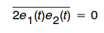
Since the noise voltages, e_1(t) and e_2(t), arise from separate resistors, they are independent, and the average of their product is zero:
E[2 * e_1(t) * e_2(t)] = 0
이때 노이즈 전압 e_1(t)과 e_2(t)는 서로 다른 저항에서 발생하므로 독립적이며, 따라서 두 값의 곱에 대한 평균은 0이 됩니다:
E[2 * e_1(t) * e_2(t)] = 0
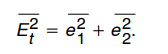
This results in
E_t^2 = e_1^2 + e_2^2
그 결과 다음과 같은 식이 도출됩니다:
E_t^2 = e_1^2 + e_2^2
Therefore, as long as the noise sources arise from separate mechanisms and are independent, which is usually the case, the average mean square value of a sum of separate independent noise sources is the sum of the individual average mean square values. Thus in our example E_t^2 = \int 4kT(R_1 + R_2)df, which is what would be expected. This is derived using voltage sources, but also is true for current sources. The same result can be shown to be true when considering two independent sine wave sources.
그러므로 노이즈원들이 서로 다른 메커니즘에서 발생하고 독립적이기만 하다면(보통의 경우가 이에 해당합니다), 분리된 독립 노이즈원들 합의 평균 제곱값은 각각의 개별 평균 제곱값들의 합과 같습니다. 따라서 본 예시의 경우, 예상했던 대로 E_t^2 = \int 4kT(R_1 + R_2)df가 됩니다. 이 결론은 전압원을 사용하여 도출되었지만 전류원에도 동일하게 적용됩니다. 두 개의 독립적인 사인파(sine wave) 소스를 고려할 때도 동일한 결과가 성립함을 보일 수 있습니다.

목차 확인
https://brush-up.tistory.com/431
Noise Analysis inOperational Amplifier Circuits(1)
아래 문서 내용에 대한 번역 및 정리이다. https://www.ti.com/lit/an/slva043b/slva043b.pdf?ts=1780557822918&ref_url=https%253A%252F%252Fwww.google.com%252F Noise Analysis in Operational Amplifier Circuits연산 증폭기(Op-Amp) 회로에서
brush-up.tistory.com
'시스템 반도체 설계 > Amplifier' 카테고리의 다른 글
| Noise Analysis in Operational Amplifier Circuits (3) Types of Noise (0) | 2026.06.06 |
|---|---|
| Noise Analysis in Operational Amplifier Circuits (2) (0) | 2026.06.05 |
| Noise Analysis inOperational Amplifier Circuits(1) (0) | 2026.06.04 |